Wagner–Whitin Revisited: Optimal Inventory Planning Without Guesswork
Reducing inventory without hurting service levels is one of the hardest problems in operations. While many organizations rely on heuristics or rules of thumb, there is a lesser-known but mathematically exact solution for a very common planning scenario: the Wagner–Whitin algorithm.
In this article, we look at what the Wagner–Whitin problem is, where it works best, its limitations, and how realistic it is to embed it into modern BI or ERP environments.
What Is the Wagner–Whitin Problem?
The Wagner–Whitin problem (1958) is a dynamic lot-sizing model designed for a single item over a finite planning horizon.
Its goal is simple: Minimize total cost = setup (ordering) cost + inventory holding cost…
…while meeting known future demand exactly and allowing inventory to be carried between periods.
Key assumptions
- Deterministic demand (you know future demand)
- Single product
- No backorders allowed
- Fixed ordering (setup) cost
- Linear holding cost
- Finite time horizon
Despite these constraints, the model is provably optimal for this setting.
Where Is Wagner–Whitin Used in Practice?
Although it is often presented as a “textbook” algorithm, Wagner–Whitin (or its extensions) is used in:
1. Retail replenishment planning
- Seasonal or promotional products
- Short-term SKU-level planning
- Central warehouses supplying stores
2. Manufacturing & MRP logic
- Production planning with setup costs
- Make-to-stock environments
- Component-level lot sizing
3. Inventory analytics & BI layers
- What-if simulations
- Policy benchmarking (heuristics vs optimal)
- Cost-to-serve analysis
In many real systems, heuristics approximate Wagner–Whitin, but few teams ever measure how far they are from the theoretical optimum.
Why It Matters: Inventory Reduction Potential
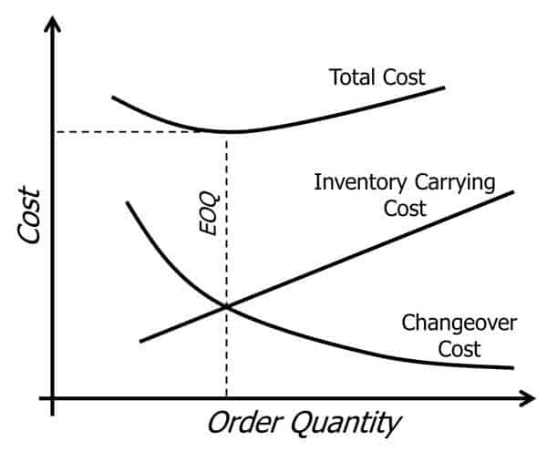
In practice, comparing heuristic policies (EOQ, fixed cycle, min–max) against Wagner–Whitin often shows:
- 5–15% inventory reduction
- Lower peak inventory
- Better alignment of orders with demand structure
A “10% average inventory reduction” is absolutely realistics, especially in retail.
Example: A Hypothetical Warehouse
Below are three simple visualizations based on a hypothetical 10-period demand scenario.
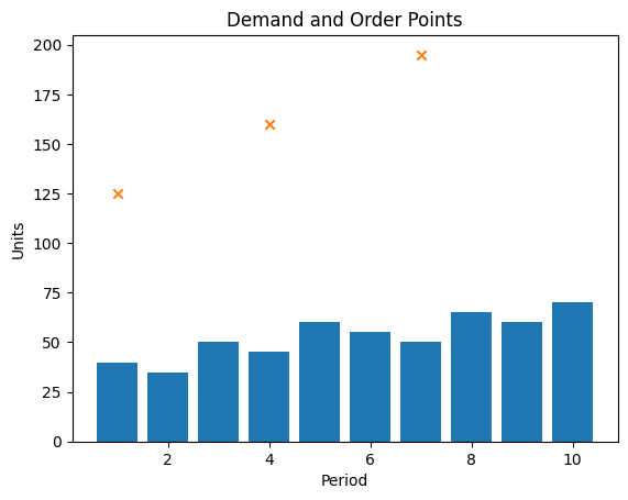
1. Demand over time
This shows fluctuating but fully known demand across periods.
Interpretation:
Demand is uneven — exactly the situation where fixed order quantities perform poorly.
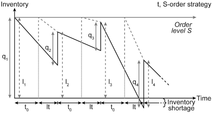
2. Inventory levels under optimal lot sizing
Here we see inventory levels resulting from an optimized order plan.
Interpretation:
- Inventory builds up only when economically justified
- Stock reaches zero exactly before new orders
- No “just in case” buffers
This is the mathematical definition of inventory discipline.
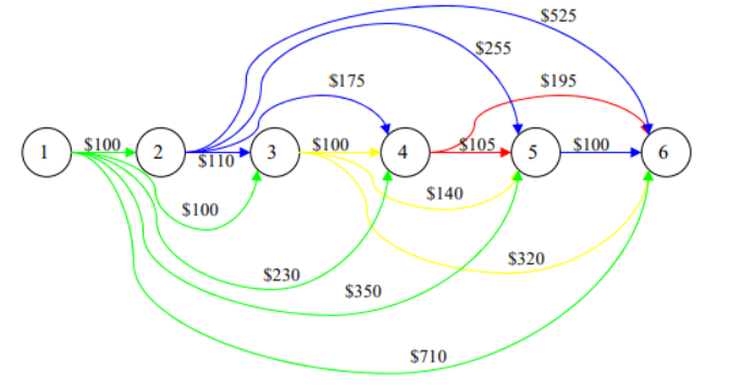
3. Demand and order points
Interpretation:
- Orders are placed only in selected periods
- Each order covers multiple future periods
- The timing is cost-optimal, not calendar-based
Is It “Too Simple” to Be Useful?
hort answer: no — but it must be used correctly.
Strengths
- Exact optimal solution
- Transparent logic
- Excellent benchmark
- Works well for short- to mid-term planning
Limitations
- Requires reliable demand forecasts
- Single-item focus
- No capacity constraints
- Not stochastic
This makes it ideal for analytics and decision support, and less suitable as a standalone operational system.
Python Implementations
Wagner–Whitin is very well supported in Python.
Common approaches:
- Dynamic programming (custom implementation)
- Linear programming (PuLP, Pyomo)
- Integration into planning notebooks
Typical workflow:
- Pull demand from ERP
- Run optimization in Python
- Push recommendations back as planning inputs
ERP & BI Integration: Is It Realistic?
Very much so.
A common architecture:
- ERP remains the system of record
- Python/BI layer computes optimal plans
- Results feed:
- reorder proposals
- safety stock calibration
- scenario analysis dashboards
Wagner–Whitin works best as a decision engine, not a replacement ERP module.