Inventory Management for Retail Under Stochastic Demand – Key Takeaways
This is a review of Inventory Management for Retail – Stochastic Demand by Samir Saci (https://towardsdatascience.com/inventory-management-for-retail-stochastic-demand-3020a43d1c14/). All the graphs were also created by the Author, Samir Saci.
Retail inventory managers often rely on simple, rule-based replenishment policies built into ERPs, but real demand is uncertain — it fluctuates. Acknowledging randomness in demand and evaluating its impact systematically can significantly change how inventory is planned and controlled.
Why Stochastic Demand Matters
In the real world, demand isn’t a fixed number (e.g., “100 units per week”). Instead, it varies due to customer behavior, seasonality, promotions, and random fluctuations. Modeling demand as a random variable — for example, normally distributed — brings a more realistic foundation to inventory decisions than treating it as a known constant.
In a typical scenario for a mid-size retail chain:
- The inventory manager must set replenishment rules in the ERP,
- Standard rules might lead to stock-outs for fast-moving items,
- and traditional deterministic assumptions hide the risk caused by variability.
Classic Replenishment Rules Fall Short
The article contrasts deterministic approaches (assume known demand) with stochastic modeling. With deterministic demand, you might compute reorder points and quantities directly based on fixed figures. But when demand is stochastic (random), you need methods that incorporate variability explicitly into safety stock and order policies.
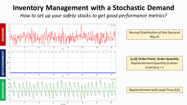
Continuous Review Policy: (s, Q)
One of the main policies discussed in the article is the continuous review (s, Q) model:
- You monitor inventory continuously,
- When it falls to a threshold s, you order a fixed quantity Q.
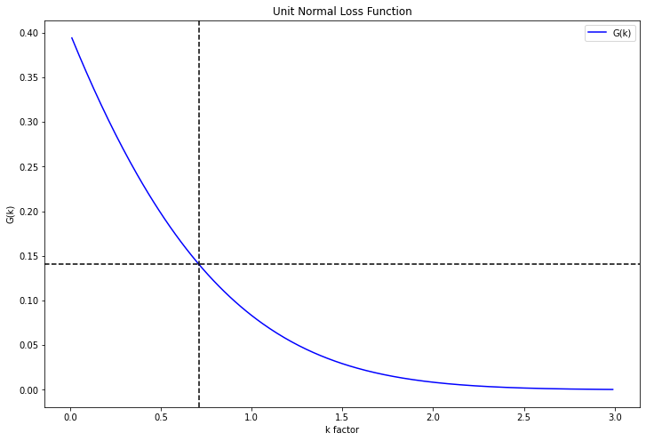
Under stochastic demand, the reorder point (s) isn’t just the average demand during lead time — it must also include safety stock to buffer against uncertainty. To determine safety stock, the policy uses a standard normal distribution assumption and a multiplier k depending on service level targets (like 95% or 99%).
Two key metrics:
- Cycle Service Level (CSL) – probability of avoiding stock-outs in a cycle,
- Item Fill Rate (IFR) – proportion of demand satisfied without stock-out.
These help tie statistical modeling directly to business performance.
What the Model Shows (Example Highlights)
The article walks through examples where demand is assumed normally distributed with a mean and variance. It calculates:
- how safety stock and reorder points change with higher service level goals,
- how the choice of k affects inventory and fill rates.
For instance:
- targeting CSL = 95% might require different safety stock than
- targeting IFR = 99%, even with the same average demand.
This kind of analysis is crucial for retailers because it quantifies trade-offs between higher service and higher holding costs.
Business Takeaways
For practitioners and analysts, here’s what matters most:
✅ Don’t assume demand is constant.
Uncertainty affects reorder points and safety stock — and impacts service levels and costs.
✅ Continuous review models can improve service but may be operationally expensive.
✅ Periodic review policies are often more practical at scale.
✅ Quantifying service level targets (CSL, IFR) clarifies the value of holding extra inventory versus the cost of stock-outs.One of the main policies discussed in the article is the continuous review (s, Q) model: