Case Study: Machine Learning–Driven Cash-Flow Forecasting for ATM Operations
Executive Summary
The error reduction (measured via MAE) directly translates into more precise cash planning
The weekday seasonality view gives operations an immediate rule-of-thumb: which days require systematically higher limits or earlier refills.
The scatterplot reassures risk and analytics teams that the model is not just good on average, but behaves sensibly across low, medium, and high-demand days.
Business Problem & Why Forecast Accuracy Matters
For retail banks and ATM operators, cash logistics is one of the most capital-intensive and operationally sensitive processes. Each ATM must carry enough cash to avoid service disruptions, yet overstocking leads to excessive working capital, unnecessary CIT (cash-in-transit) operations, and higher insurance costs.
Even small improvements in forecast accuracy can translate into significant operational savings. A 10% reduction in forecast error may reduce annual cash logistics costs by 5–8%, depending on fleet size and replenishment frequency.
The client — a regional ATM operator — wanted a data-driven forecasting system that could outperform their existing rule-based predictions and enable
Our goal: produce a reliable 30-day ahead forecast of daily ATM cash withdrawals, with model transparency and automated deployment.
- fewer emergency replenishments,
- better liquidity planning,
- lower idle cash,
- and improved customer service availability.
Data & Methods
The project used a historical dataset of daily ATM withdrawal amounts.
Key components included:
- Daily total cash withdrawals over ~12 months
- Calendar-based effects: weekdays, weekends, holidays
- Seasonal cycles: end-of-month patterns, salary periods
- Outlier events: sudden spikes due to local promotions or system outages
- Weather & mobility proxies: optional, but correlated for some sites
The raw dataset required several preprocessing steps, including:
- outlier detection and capping,
- handling missing values during ATM downtime,
- smoothing abnormal spikes due to rare events,
- feature engineering for trend, seasonality, and lagged effects.
The resulting modeling dataset consisted of
- a clean, stationary time series suitable for machine learning.
- ~365 rows (daily observations),
- ~20 engineered features.
Modeling Approach & Technical Considerations
We compared multiple time-series forecasting methods:
Baseline Models
- Moving average & exponential smoothing
- Classical Holt–Winters
Intermediate Models
- ARIMA / SARIMA
Provided stronger temporal structure modeling, but struggled with volatility and non-linear withdrawal patterns.
Good for benchmarking, but limited in capturing irregular seasonality.
Advanced Model (Final Winner): Random Forest Regressor
Although Random Forest is not a classical time-series model, it performs exceptionally well on feature-engineered temporal datasets, capturing non-linear relationships and interactions.
Key features used by the model:
- Lag features: t-1, t-2, t-7, t-14
- Rolling means: 7-day, 14-day
- Rolling volatility
- Day-of-week, day-of-month, month
- Salary-period indicators
- Holiday & event flags
Technical implementation highlights:
- Hyperparameter tuning via RandomizedSearchCV
- Out-of-sample validation on the final 30 days
- Error metrics: MAE, RMSE, MAPE
- Feature importance analysis for explainability.
Results / Charts
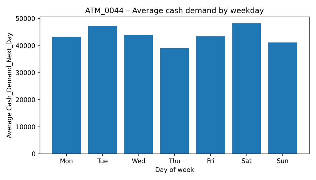
Average Next-day cash demand
A bar chart of average next-day cash demand by weekday.
This highlights systematic calendar effects (e.g. certain weekdays consistently higher or lower), which are crucial for refill scheduling and staffing.
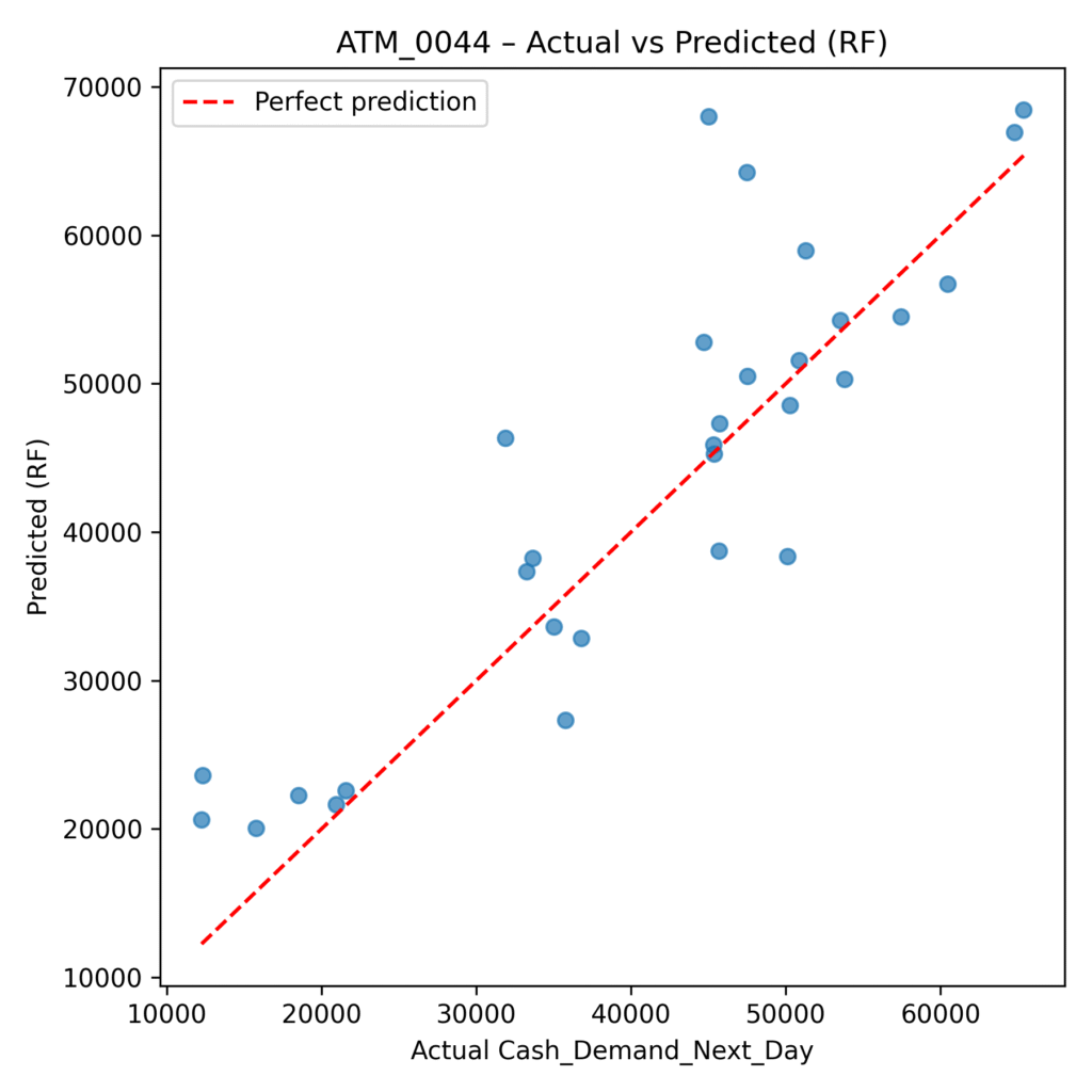
Actual vs Predicted Scatterplot
A scatter of y_test (actual) vs y_pred_rf (RF predictions), with a dashed 45° line indicating perfect forecasts.
Points tightly clustered around the diagonal indicate a well-calibrated model; systematic deviations would reveal bias (e.g. underpredicting high-demand days).
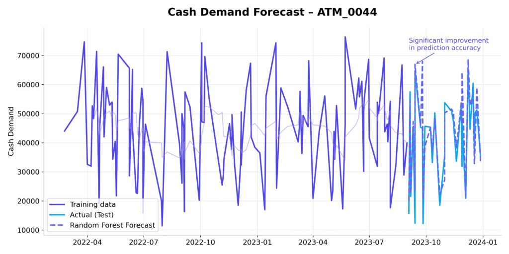
History & forecast chart
A line chart showing:
- Historical training period (actual cash demand)
- Test period (actual demand)
- Random Forest forecast on the test period..
This makes it immediately visible where the model tracks reality closely and where deviations occur.
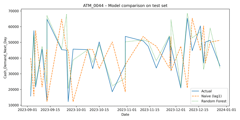
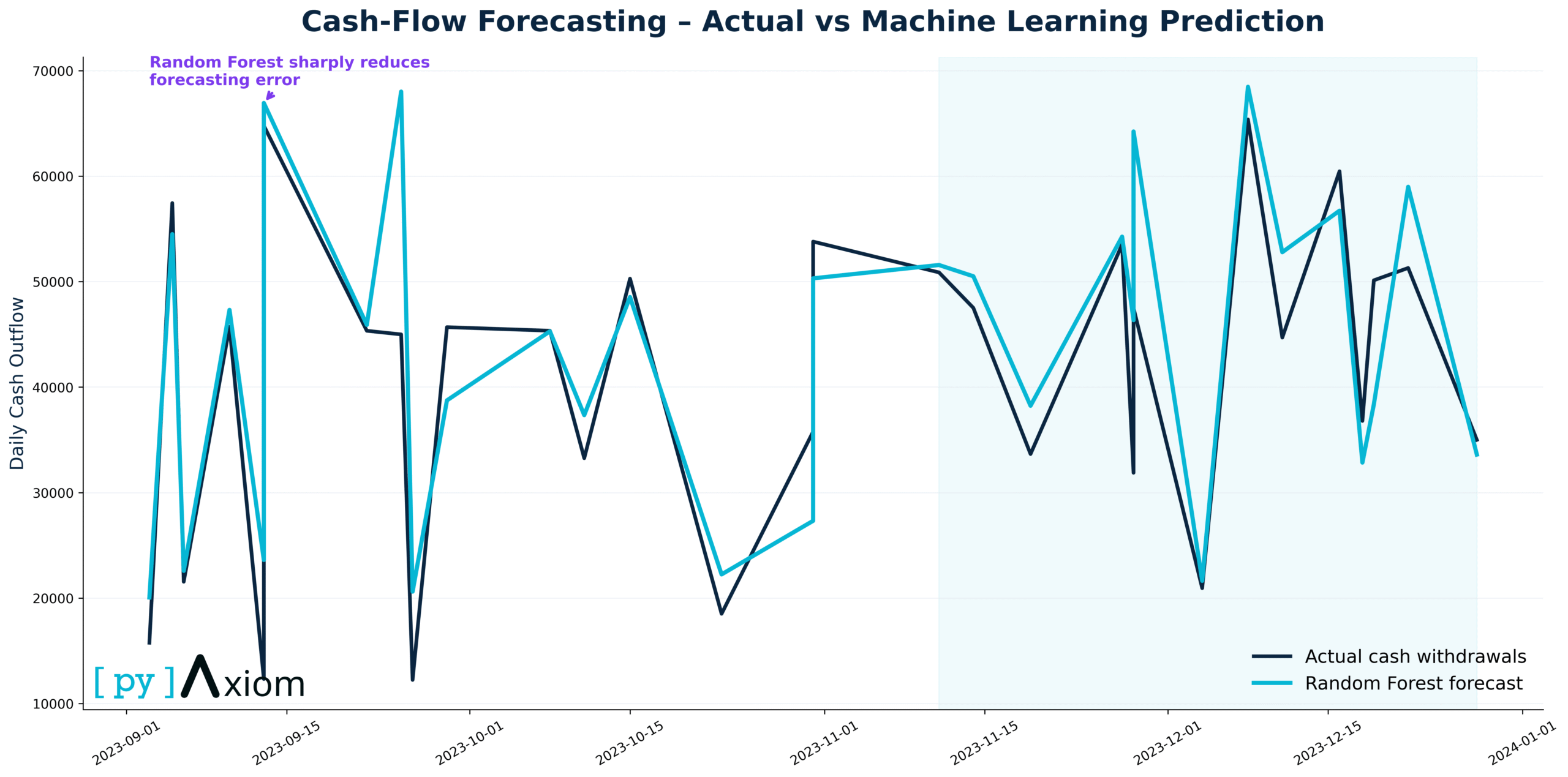
Model Comparison on the Test Set
Another line chart, but now overlaying three series on the 30-day test window:
- Actual demand
- Naïve forecast (lag1)
- Random Forest forecast
This is the key visual to demonstrate value: the RF line typically sticks closer to the actual curve and reacts better to shifts than the naïve model.
Business Impact
From a business standpoint, this is the essence of BI-supported fraud and risk management:
- Even a relatively simple machine-learning model using basic transactional, calendar, and lagged features can materially outperform a naïve “yesterday = tomorrow” rule.
- The error reduction (measured via MAE) directly translates into more precise cash planning:
- fewer emergency refills and stock-outs,
- less idle cash trapped in ATMs,
- smoother logistics for cash-in-transit teams.
- Operational efficiency — as manual review teams focus their effort exactly where it adds most value.The weekday seasonality view gives operations an immediate rule-of-thumb: which days require systematically higher limits or earlier refills.Operational efficiency — as manual review teams focus their effort exactly where it adds most value.
- The scatterplot reassures risk and analytics teams that the model is not just good on average, but behaves sensibly across low, medium, and high-demand days.
- The final chart summarizes the story for non-technical stakeholders: historical performance, model forecasts, and the qualitative message that “machine learning brings ATM cash forecasting under control.
This case study forms a concrete, data-driven example of how pyAxiom can help finance and operations teams move from static rules to intelligent, learning-based cash-flow forecasting – starting with a single ATM and easily scaling to large networks.